Time Series & Forecasting

A “Bachelorette” Prediction App Taught Me Why Naive Forecasting Models Break on Seasonal Data

Independent project — Time Series Analysis course (Business Analytics)Senior year, spring semesterDeployed — 5 live Shiny apps on shinyapps.ioR (fpp3, forecast, tsibble), Shiny, Google Trends data

~245 monthly Google Trends data points modeled7 forecasting models compared (Mean, Naive, Drift, Seasonal Naive, TSLM, ETS, ARIMA)5 apps deployed live on shinyapps.ioIndependent project, Time Series Analysis course

Context

What the system looked like before.

After I presented the CTCF poster, I left Dr. McCord's lab and started my senior year. I took a business analytics stats class on Time Series Analysis — model building techniques for linear time series, univariate forecasting, Box-Jenkins methods, exponential smoothing, autoregression, and forecasting from regression models. It was a higher-level course for business analytics majors and I felt like a fish out of water.

Question

Can simple forecasting models predict something as spiky and seasonal as public interest in a reality TV show — or does that kind of data demand something more than a naive baseline?

Approach & rationale

Our midterm was predicting viewer trends. I built an interactive app attempting to predict interest in "The Bachelorette" using Google Trends data — pulling the show's monthly interest series (2004–present, ~245 data points), building it into a tsibble, and exploring it through a Shiny interface with selectable views: time series, seasonality, autocorrelation, STL decomposition, before layering forecast models on top.

Methodology & iteration

Including the paths that did not hold.

Approach A — descriptive plots only

TriedA Shiny app that reads the Google Trends data, converts it to a monthly tsibble, and lets the user switch between four descriptive views: raw time series, seasonality, autocorrelation, and STL decomposition.

Held upSimple linear and baseline models collapsed under the show's seasonal search spikes and required STL decomposition just to isolate true trends.

Approach B — a different kind of prediction

TriedA second app that, instead of forecasting the time series, predicts the next Bachelorette's physical characteristics by computing how often each historical value occurred.

Fell shortIt's a “prediction” in name only — an empirical-frequency lookup, not a forecasting model — useful as a contrast to the time-series work, not a replacement for it.

Final approach — combined, and debugged

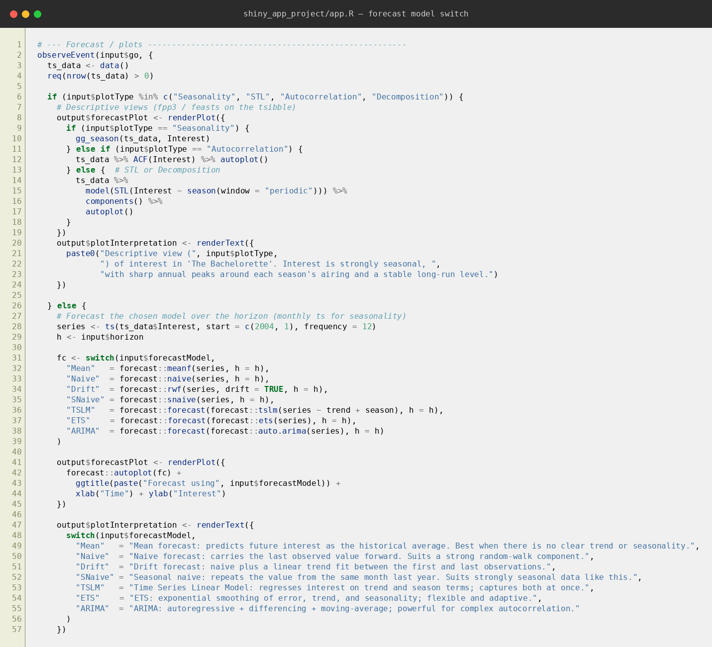
TriedThe two apps were merged into one: seven real forecasting models (Mean, Naive, Drift, Seasonal Naive, TSLM, ETS, ARIMA) over a user-chosen horizon, alongside the descriptive views and the characteristics predictor.

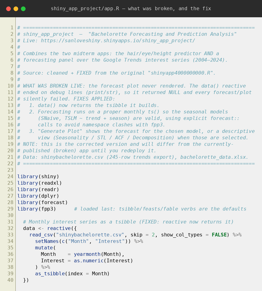
Fell shortA concrete bug: the deployed forecast plot silently failed because its data-loading reactive ended on debug lines instead of returning the tsibble, so every downstream forecast got NULL.

Held upThe fix: making the reactive actually return the tsibble, and running the forecast models on a proper monthly ts() object so the seasonal models (SNaive, TSLM) had valid frequency information.

Code diff showing the broken forecast reactive and its fix — The broken reactive — debug lines instead of a return — and the fix.

In short

Results

Numbers first, not buried in prose.

My predictions highlighted the exact shortcomings we studied in class, as simple linear and baseline models collapsed under the show's seasonal search spikes and required STL decomposition just to isolate true trends. Those mistakes were what I needed — it demystified the mathematical mechanics behind signal processing and showed me how easily naive assumptions can distort predictions.

The app lets a viewer pick a model interactively rather than reporting a single quantitative winner — it's exploratory, not a verdict on which model performed best.

Seven forecasting models shown side by side in the deployed app — The final app's seven-model forecast switch, side by side.

Significance

Where this went.

Five apps live and running on shinyapps.io as of the last deployment check: the combined forecasting app, both midterm apps, and two smaller course exercises.

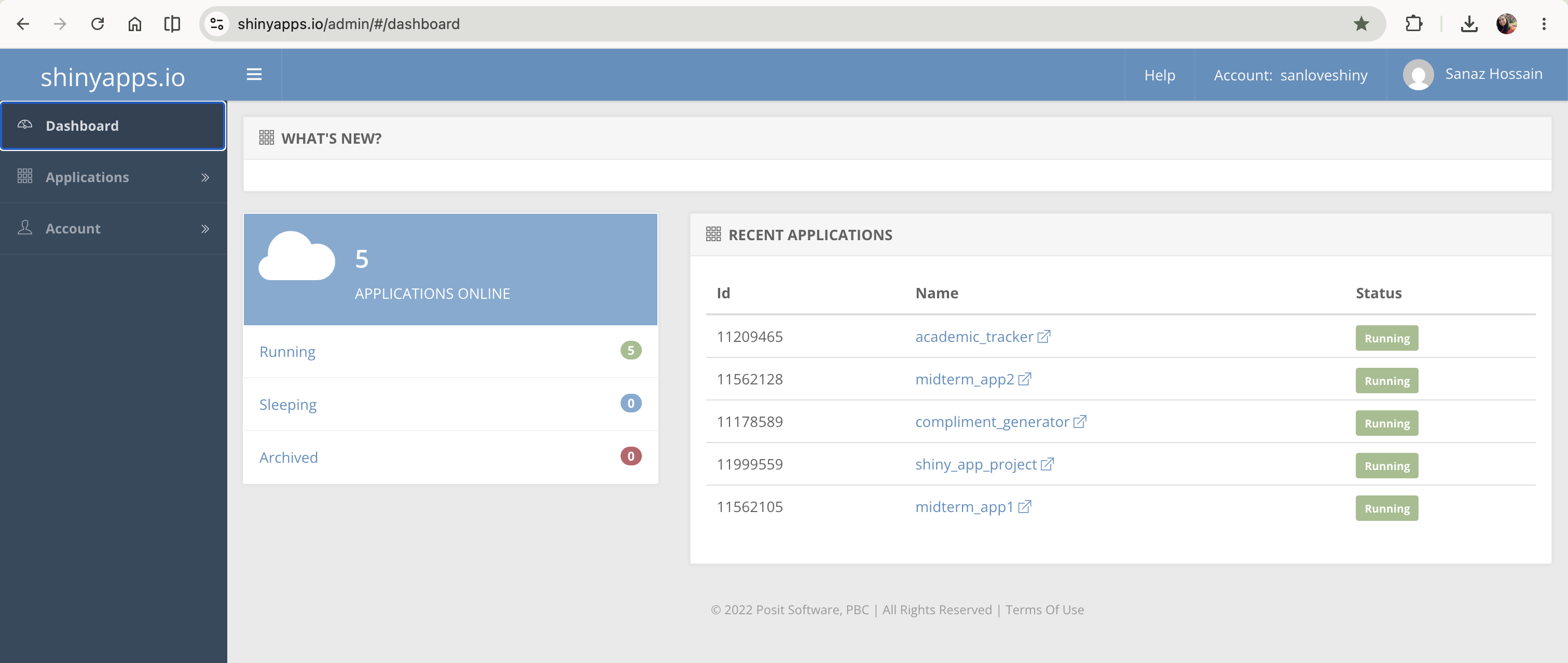
shinyapps.io dashboard showing five apps live — All five apps live on shinyapps.io.

Reflection

While predicting television search trends and tracking DNA damage seem worlds apart, both sets of data points showed me the same thing: a surge in popularity one week carries momentum into the next, the same way genomic sections at varying distances from an induced cut site carry the residue of that damage. Just as television ratings from one week depend heavily on the week before, the structural integrity of a DNA sequence depends heavily on how close it sits to a physical break.

BackAll work NextMolecular Docking →